Mini-batch multiplicative updates for NMF with \(\beta\) -divergence
In [1] we propose mini-batch stochastic algorithms to perform NMF efficiently on large data matrices. Besides the stochastic aspect, the mini-batch approach allows exploiting intesive computing devices such as general purpose graphical processing units to decrease the processing time further and in some cases outperform coordinate descent approach.
NMF with \(\beta\) -divergence and multiplicative updates
Consider the (nonnegative) matrix \(\textbf{V}\in\mathbb{R}_+^{F\times N}\). The goal of NMF [2] is to find a factorisation for \(\textbf{V}\) of the form:
where \(\textbf{W}\in\mathbb{R}_+^{F\times K}\) , \(\textbf{H}\in\mathbb{R}_+^{K\times N}\) and \(K\) is the number of components in the decomposition. The NMF model estimation is usually considered as solving the following optimisation problem:
Where \(D\) is a separable divergence such as:
with \([.]_{fn}\) is the element on column \(n\) and line \(f\) of a matrix and \(d\) is a scalar cost function. A common choice for the cost function is the \(\beta\) -divergence [3] [4] [5] defined as follows:
Popular cost functions such as the Euclidean distance, the generalised KL divergence [6] and the IS divergence [7] and all particular cases of the \(\beta\)-divergence` (obtained for \(\beta=2\) , \(1\) and \(0\), respectively). The use of the \(\beta\) -divergence for NMF has been studied extensively in Févotte et al. [8]. In most cases NMF problem is solved using a two-block coordinate descent approach. Each of the factors \(\textbf{W}\) and \(\textbf{H}\) is optimised alternatively. The sub-problem in one factor can then be considered as a nonnegative least square problem (NNLS) [9]. The approach implemented here to solve these NNLS problems relies on the multiplicative update rules introduced in Lee et al. [2] for the Euclidean distance and later generalised to the the \(\beta\) -divergence [9] :
where \(\odot\) is the element-wise product (Hadamard product) and division and power are element-wise. The matrices \(\textbf{H}\) and \(\textbf{W}\) are then updated according to an alternating update scheme.
Mini-batch multiplicative updates for NMF
The standard update scheme requires the complete matrix \(\textbf{V}\). When considering time series with a large number of data points(or time series that are expending in time) running this algorithm can become prohibitive. Capitalising on the separability of the divergence (2) it is possible to perform NMF on mini-batch of data to reduce to computational burden of to allow for parallel computations [10].
When considering time series as defined above, each column (\(V_i\)) of the matrix \(\textbf{V}\) contain all the features for a specific time frame and each row represent a particular feature along time. The number of row is then a parameter of the low-level representation and only the number of columns can increase while increasing the amount of data. Therefore, in contrast to the approach proposed by Simsekli et al. [10] we decide to decompose the matrix \(\textbf{V}\) in \(B\) mini-batches of time frames that contains all the features for the given frame.
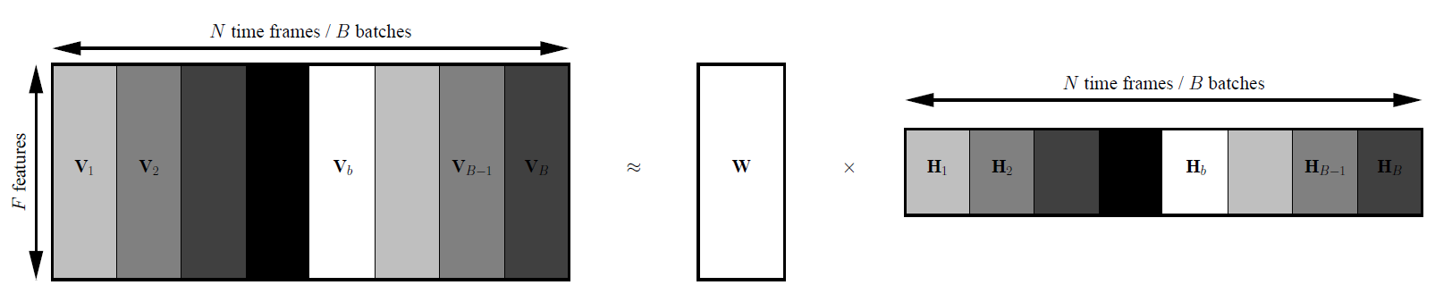
Fig. 1 Mini-batch decomposition of the data matrix \(\textbf{V}\)
For each batch \(b\), the update of the activations \(\textbf{H}_b\) corresponding to \(\textbf{V}_b\) can be obtained independently from all the other batches with the standard MU~eqref{upH}. The update of the bases \(\textbf{W}\) on the other hand require the whole matrix \(\textbf{V}\) to be processed. The positive contribution of the gradient (nabla^+textbf{W}) and the negative contribution of the gradient \(\nabla^-\textbf{W}\) are accumulated along the mini-batches. \(\textbf{W}\) is updated once per epoch with the standard MU rule (4) as described in Algorithm [1]. Note that this is theoretically similar to the standard full-gradient (FG) MU rules.
Stochastic mini-batch updates
When aiming at minimizing an Euclidean distance, it has been shown than drawing samples randomly can improve greatly the convergence speed in dictionary learning and by extension in NMF [11] [12]. We propose to apply a similar idea to MU in order to take advantage of the wide variety of divergences covered by the \(\beta\)-divergence. Instead of selecting the mini-batch sequentially on the original data \(\textbf{V}\) as above, we propose to draw mini-batches randomly on a shuffled version of \(\textbf{V}\). The mini-batch update of \(\textbf{H}\) still need one full pass through the data but a single mini-batch can be used to update \(\textbf{W}\), in an way analogous to stochastic gradient (SG) methods [13].
Two different strategies can be considered to updates \(\textbf{W}\). The first option is to updates \(\textbf{W}\) for each mini-batch, this approach is denoted asymmetric SG mini-batch MU (ASG-MU) as \(\textbf{H}\) and \(\textbf{W}\) are updated asymmetrically (the full \(\textbf{H}\) is updated once per epoch while \(\textbf{W}\) is updated for each mini-batch). The second option is to update \(\textbf{W}\) only once per epoch on a randomly selected mini-batch a described this approach will be referred to as greedy SG mini-batch MU (GSG-MU). Detailled description of the algorithm can be found in [1]
Stochastic average gradient mini-batch updates
Stochastic average gradient (SAG) [14] is a method recently introduced for optimizing cost functions that are a sum of convex functions (which is the case here). SAG provide an intermediate between FG-like methods and SG-like methods. SAG then allows to maintain convergence rate close to FG methods with a complexity comparable to SG methods.
We propose to apply SAG-like method to update the dictionaries \(\textbf{W}\) in a mini-batch based NMF. Note that, as the full pass through the data is needed to update \(\textbf{H}\) it would not make sense to apply SAG here. The key idea is that for each mini-batch \(b\) instead of using the gradient computed locally to update \(\textbf{W}\), we propose to use the mini-batch data to update the full gradient negative and positive contributions:
where \(\nabla^-_{\mathrm{new}}\textbf{W}_b\) and \(\nabla^+_{\mathrm{new}}\textbf{W}_b\) are the negative and positive contribution to the gradient of \(\textbf{W}\) calculated on the mini-batch \(b\), respectively. \(\nabla^-_{\mathrm{old}}\textbf{W}_b\) and \(\nabla^+_{\mathrm{old}}\textbf{W}_b\) are the previous negative and positive contribution to the gradient of \(\textbf{W}\) for the mini-batch \(b\), respectively.
Similarly as above, two different strategies can be considered to updates \(\textbf{W}\). The first option is to updates \(\textbf{W}\) for each mini-batch this approach is denoted asymmetric SAG mini-batch MU (ASAG-MU). The second option is to update \(\textbf{W}\) only once per epoch on a randomly selected mini-batch which is greedy SAG mini-batch MU (GSAG-MU). Detailled description of the algorithm can be found in [1]
Download
Source code available at https://github.com/rserizel/minibatchNMF
Getting Started
A short example is available as at https://github.com/rserizel/minibatchNMF/blob/master/minibatch_BetaNMF_howto.ipynb
Citation
If you are using this source code please consider citing the following paper:
Reference
- Serizel, S. Essid, and G. Richard. “Mini-batch stochastic approaches for accelerated multiplicative updates in nonnegative matrix factorisation with beta-divergence”. Accepted for publication In Proc. of MLSP, p. 5, 2016.
Bibtex
@inproceedings{serizel2016batch,
title={Mini-batch stochastic approaches for accelerated multiplicative updates in nonnegative matrix factorisation with beta-divergence},
author={Serizel, Romain and Essid, Slim and Richard, Ga{“e}l},
booktitle={IEEE International Workshop on Machine Learning for Signal Processing (MLSP)},
pages={5},
year={2016},
organization={IEEE} }
References
| [1] |
|
| [2] |
|
| [3] |
|
| [4] |
|
| [5] |
|
| [6] |
|
| [7] |
|
| [8] |
|
| [9] |
|
| [10] |
|
| [11] |
|
| [12] |
|
| [13] |
|
| [14] |
|